Study on Gemma-2-2B-IT

TL;DR:
LLMs internally represents the correct way to compare numbers (80–90% accuracy in penultimate layers) but the final layer corrupts this knowledge, causing simple failures like 9.8 < 9.11.

---

Executive Summary

The Problem: A paradox in LLM Capabilities

LLMs can ace complex reasoning yet still fail at simple numeric comparisons like 9.8 < 9.11. Using Gemma-2-2B-IT, I ask: Does the model internally represent the correct Yes/No decision, and if so, where does the failure happen? This matters because robust numeric comparison is a prerequisite for any downstream task that relies on arithmetic or ordering.

High-level takeaways

The representation is good; the output is bad. Mid/late layers encode a clean Yes/No separation (80–90% forced-choice accuracy using internal signals without any training), but the final layer corrupts it, especially for decimals ⇒ systematic Yes-bias and errors on “No” cases.

Length heuristic is real. integers_diff_len relies on a direction partially misaligned with other numeric sets, consistent with “shortcut” reliance on length. Fastest to learn the correct internal representation to compare the two integers with different length.

Last-layer MLP is the culprit. Causal patching L24→L25 (at mlp_post / resid_post) improves accuracy by a lot; other patches hurt or are neutral.

Small, targeted ablations work. Disabling ~50 harmful neurons at the final block meaningfully improves accuracy—largest gains for integers_equal_len and decimals_diff_len. Even removal of ~10 harmful neurons gave a good boost for accuracy, though lesser than removing 50 harmful neurons.

---

Key Results

1) Geometry shows the model “knows” the answer

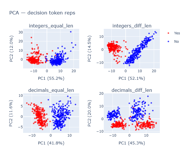
What: PCA on last-layer hidden states per dataset; color by truth. Finding: Numeric datasets are cleanly separable; strings aren’t. Decimals show sub-structure that becomes clearer at L-1, where accuracy is higher. Why it supports the takeaway: Separation in hidden states despite wrong outputs implies a output projection failure, not a representation failure.

2) Cross-dataset axis alignment reveals a shared comparator (except length)

What: Compute the Yes–No mean-difference axis per dataset/layer; compare axes via cosine similarity. Finding: Most numeric sets align strongly (>0.85), but integers_diff_len is least aligned (~0.6), consistent with a length-based heuristic distinct from value comparison. Why: A shared axis suggests a common value comparator subspace; misalignment flags a different (shortcut) mechanism.

3) Readout vs representation: forced-choice along the unembedding direction

What: Project layer activations onto the Yes–No unembedding direction and compute forced-choice accuracy per layer. Finding: Accuracy is near random until ~L23, then peaks, then collapses at L25, with the strongest failure on decimal “No” cases (systematic Yes-bias). Why: The late readout step (not the earlier representation) drives the error, pinpointing where to intervene.

4) Causal edits: last-layer MLP corrupts the decision

What: Activation patching from L24→L25 at multiple hooks using TransformerLens Nanda & Bloom, 2022. Finding: Patching mlp_post/resid_post improves accuracy; other patches often hurt. Why: This isolates the final-block MLP as the primary corruption source.

5) Targeted neuron ablations repair failures

What: Rank final-block neurons by gradient-weighted contribution to the Yes–No margin; ablate the top-50 harmful globally and per-dataset. Finding: Large gains for integers_equal_len and decimals_diff_len; residual asymmetries show the model still attends to decimal length when truth is “No”. Why: Confirms that a small, surgical set of neurons drive the bias—and that fixing them restores behavior.

Bottom line

Gemma-2-2B-IT internally represent the correct comparator but the last-layer MLP (readout) introduces a Yes-biased corruption. Simple, principled interventions—patching or ablating ~50 neurons—substantially reduce errors, and diagnostics suggest a lingering length heuristic distinct from true value comparison.

---

Table of Contents

• 1. Motivation
• 2. Dataset & Setup
• 3. Part I — Geometry & Emergence
• 4. Part II — Readout vs Representation
• 5. Part III — Causal Edits (Patching & Ablations)
• 6. Discussion
• 7. Repro Notes
• 8. Limitations & Next Steps

---

1. Motivation

Large Language Models (LLMs) have demonstrated Olympiad-level performance in complex reasoning, yet they paradoxically stumble on fundamental operations like basic numeric comparisons 9.8 < 9.11. If a model cannot reliably perform basic numeric comparisons, its utility in downstream tasks that depend on such reasoning is severely compromised. This study investigates why a model like Gemma-2-2B-IT fails at these seemingly simple evaluations.

---

2. Dataset & Setup

Custom Dataset

To systematically probe the model’s comparison abilities, a custom dataset was created with 500 samples for each of the following categories. Each prompt followed the format: Question: Is {a} > {b}? Answer:.

The goal was to:

• Separate numeric from lexicographic comparisons.
• Disentangle length cues while doing value comparison.
• Provide a control (strings) for lexicographic comparisons.

Created a custom dataset with 500 samples for each in the format Question: Is {a} > {b}? Answer:

• Integers (Equal Length): Question: Is 8719 > 9492? Answer:
• Integers(different length) Question: Is 526 > 1080? Answer:
• Decimals (equal length, same integer part) Question: Is 56.680 > 56.656? Answer:
• Decimals (different length, same integer part) Question: Is 37.69 > 37.4? Answer:
• Strings (equal length) Question: Is zxqahuuf > takpmzhf? Answer:
• Strings (different length) Question: Is iuygoqmivd > xzczm? Answer:

Forced-Choice Output

To isolate the comparison logic, the model’s output was restricted to only the “Yes” and “No” tokens. The logits for all other tokens were set to negative infinity, effectively forcing a binary choice and allowing us to analyze the model’s confidence between the two.

Terminology and Assumptions:

• Layer indexing is starting from 0. Model has total 26 transformer block, will be referred as 0 to 25. I also have used -1 to describe the input embedding for some of the graphs, as the hf library includes the input embedding as the first layer.
• Integers (Equal Length) => integers_equal_len; Integers(different length) => integers_diff_len; Decimals (equal length, same integer part) => decimals_equal_len; Decimals (different length, same integer part) => decimals_diff_len
• Readout : how you turn internal representations into the final prediction; the final mapping that converts that geometry into the emitted token.

Baseline Performance

The model’s baseline accuracy reveals a significant bias, especially in decimal comparisons.

Note: accuracy is specific to that particular bucket of Pair Type and True Answer.

Pair Type	True Answer	Count	Accuracy (%)
decimals_diff_len	No	246	15%
	Yes	254	100.0%
decimals_equal_len	No	264	5%
	Yes	236	100.0%
integers_diff_len	No	255	71.0%
	Yes	245	99.0%
integers_equal_len	No	267	74.0%
	Yes	233	99.0%
string_diff_len	Yes	268	13.0%
	No	232	85.0%
string_equal_len	Yes	252	27.0%
	No	248	76.0%

The most striking result is the near-total failure on decimal comparisons where the correct answer is “No”. The model is overwhelmingly biased towards answering “Yes”. This led to the rejection of my initial hypothesis.

Initial Hypothesis (Rejected): I initially suspected that the model would be behaving more like string comparison for decimals as compared to integers. Reason being, the decimal comparisons are lexicographical if the length of the integer part is same, the examples I took for decimals had same integer part, so they should be compared lexicographically by model and would be more closer towards string comparison, but the model predictions for numeric vs string was totally opposite with more number of Yes for numeric vs more number of No for string. Hence the hypothesis was rejected but gave an insight that model is not getting confused between doing lexicographic comparison in decimals of equal integer part vs treating them as integer number comparisons but biased towards Yes.

Part I - Geometry & Emergence: Finding the Knowledge

3.1 PCA on hidden state activation

Goal: Test whether internal geometry separates classes even when final predictions(outputs) are wrong.

Methodology To understand the geometry of internal model’s representation we conducted a PCA on the final layer activations, for each dataset. Visualize the first two PC1 and PC2 which explained roughly >50% variance by truth and by predicted label.

• The class integers_equal_len and decimals_equal_len are separable along PC1 cleanly while the others don’t on their PC1.
• Decimals_diff_len shows a 4 sub cluster instead of 2 and when plotted for last_layer - 1 [layer 24], decimals_equal_len also started showed that subcluster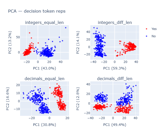
• Doing PCA on last_layer - 1 where the accuracy was high (shown ahead) had similar separation but larger magnitude in separation.
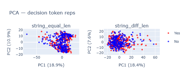
• There is no clear separation in string comparison, which explains the lack of correlation between how numeric comparison were treated as compared to string. Based on these results I thought of digging deeper into numeric only.

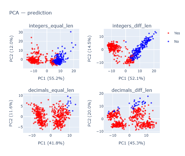
• Clearly integers has much better predictions and decimals are all Yes predictions, even when the separation is clearly evident.

3.2 Cross-Projection PCA

Goal: See if the model uses a shared mechanism for different numeric types comparison

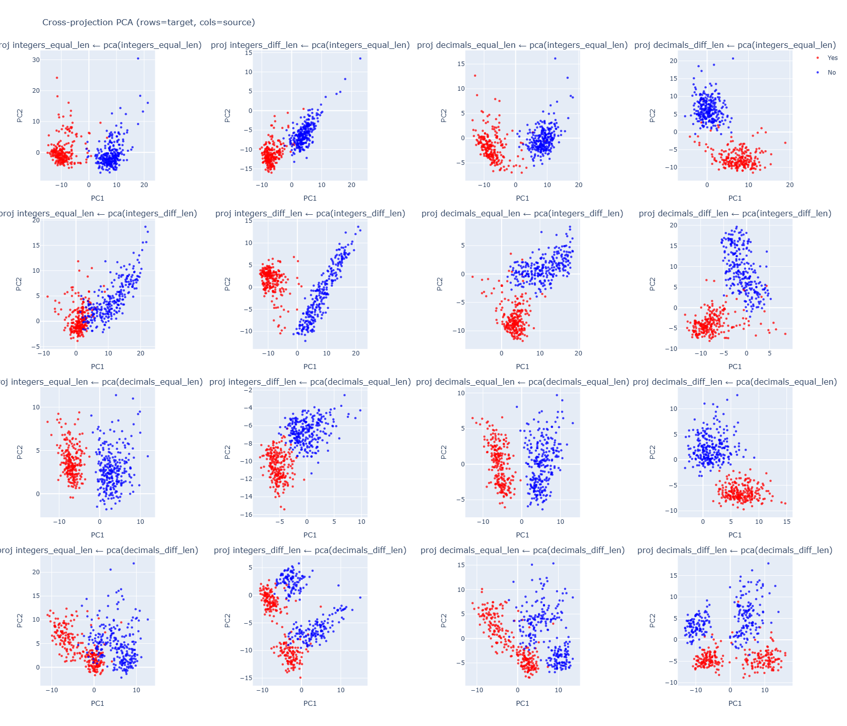
Methodology

PCA was fit on each dataset’s activations. Activations from other datasets were then projected into this learned PCA space. This helps us to ask: does a separating axis from one dataset also reveal structure in another? Answer is YES.

Calculated cosine similarity between Yes-No mean difference Appendix B axes in source vs target representations.

Cross-dataset alignment (cosine similarity)

Compute Delta_A and Delta_B for two datasets A and B (at the same layer).

Cosine similarity of their Yes–No axes

• Equivalently: align(A, B) = dot(w_A, w_B)
  • >0 ⇒ same direction (shared separator)
  • ~0 ⇒ orthogonal (unrelated)
  • <0 ⇒ opposite directions

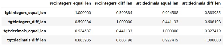
Result:

• integers_diff_len is least aligned with others (~0.6 cosine) → likely a length-based heuristic.
• Other numeric sets align strongly (> 0.85), suggesting a shared value-comparison subspace.

3.3 Cheap linear probe (difference vector)

Goal: Track where class separation emerges.

Methodology At each layer ℓ, compute unit vector w pointing from class “No” mean to “Yes” mean; measure separation Δ = |E[⟨h, w⟩ | Yes] − E[⟨h, w⟩ | No]|.

Findings:

• integers_diff_len were able to start getting separated faster than any other -> likely because it’s easy to do just based on length instead of actually comparing
• integers_equal_len started getting closer separation to integers_diff_len and decimals didn’t jump up as their integers counter part, showing there is definitely some lack of clarity as compared to integers inside LLM.
• Last Layer Collapse is a mystery, which drops the final margin suddenly when computed the margin for the last layer as compared to layer before that.

3.4 Dataset vs Dataset alignment of difference vector

Goal: See if the model uses a shared mechanism for different numeric types comparisons compared across all layers.

Methodology Check the separation direction is it same for dataset vs dataset

Dataset A = integers_diff_len Dataset B = decimals_diff_len At each layer ℓ you get two axes: 𝑤𝐴(ℓ) and 𝑤𝐵(ℓ). You then compute the cosine similarity as above: align(ℓ)(𝐴,𝐵)=⟨𝑤𝐴(ℓ),𝑤𝐵(ℓ)⟩/ ∥𝑤𝐴(ℓ)∥ ∥𝑤𝐵(ℓ)∥⟩

This is a number between –1 and 1: ≈ 1 → both datasets separate Yes vs No along the same direction at that layer. ≈ 0 → their separation axes are orthogonal (completely unrelated). ≈ –1 → they’re using opposite directions (what counts as “Yes” for one looks like “No” for the other).

Findings Clearing in we can see, integers_diff_len has a much lower correlation with other datasets, so model is definitely treating the length comparison separately and rest others in a similar manner with a high correlation of the mean diff vectors.

3.5 Trained logistic linear probes (per layer)

Goal: Quantify the linear separability of the representations at each layer

Methodology 5-fold CV logistic regression on per-layer activations; compare training per dataset vs pooled.

Findings:

• Model started learning to differentiate between integers_diff_len from layer 0
• Strong linear separability emerges mid-to-late layers; Layer 11+ cleanly separates all numeric classes.
• Tried two methods to train the regression, per dataset separately vs used a pooled dataset and trained on that and Pooled training helps decimals (positive deltas) more than it helps integers (slightly negative deltas) → shared comparator generalizes best to decimals. Thought the difference is not very high to be significant and hence seemed less interesting to me. But definitely an idea worth exploring.

4. Part II — Readout vs Representation: Finding the Failure

4.1 unembedding analysis

Goal: Project model’s activation onto it’s final output head (model.lm_head.weight). Let r = (W_u[Yes] − W_u[No]) /

(W_u[Yes] − W_u[No])

. We compute two metrics, For each layer’s activations h, compute logit gap = ⟨h, r⟩ and forced-choice accuracy = (sign(gap)) * (+1 if Yes else -1), the classification accuracy obtained by taking the sign of logit gap as the prediction multiplied by 1 if Yes else -1.

a. Logit gap: the positive value for the gap indicates bias towards Yes and negative towards No. The magnitude tells how strongly it reflects. b. Forced choice accuracy: “If model were forced to decide Yes vs No using only the activations projected at this layer, how accurate would it be? “

Findings:

• forced-choice accuracy continues to stay random till layer 22, implying the projections on r is random. I expected it to be random for all the cases surprisingly it became very high for Layer 23 and again started decreasing.

Key pattern:

1. Layer 0-2 : Decreasing bias shifts from No -> neutral.
2. Layer 3-14: slight Yes bias persist.
3. Layer 15-19: Steep Yes bias increase.
4. Layer 20-23: Bias shifts from Yes -> neutral. forced-choice accuracy peaks at Layer 23
5. Layer 24-25: Increases slightly towards yes again. accuracy drops close to random for decimals for Layer 25

Results

• This gives us an understanding that unbiased layers have higher accuracy if they also have emergence of class separation. That’s why it peaks at Layer 23 and drops back as bias started to increase again. We see emergence in previous sections and biasness in this section.

The plot shows clear indication of bias towards Yes and performance degrading from Layer 23 to Layer 25 in all 4 numeric datasets.

---

5. Part III — Causal Edits (Patching & Ablations)

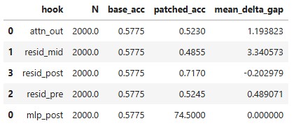
5.1 TransformerLens activation patching

Goal: Identify which sub-component corrupts the decision when moving from L24→L25.

Methodology Patch L25 activations with L24 for hooks resid_post, mlp_post, resid_pre, resid_mid, attn_out. It will help to isolate the source of the error.

Findings:

• Patching resid_post / mlp_post from L24 → L25 improves accuracy.
• Patching others often hurts.
• Interestingly the mean_delta_gap very slightly changed for which the accuracy improved but for which accuracy decreased more biasness added towards positive side. I believe that both Yes and No confidence increased equally when accuracy increased and hence mean remained close to zero.
• Result Patching the output of the MLP sub-block (resid_post, mlp_post) reliably improves accuracy. This causally implicates the final MLP layer as the primary source of corruption.

5.2 Harmful-neuron discovery & ablation

Goal: To find the minimal set of specific neurons responsible for the model’s biased failures and causally verify their impact by disabling them.

Methodology:

1. Discovery: First, I identified the most “harmful” neurons by scoring their negative impact on accuracy across the entire dataset. Neurons were ranked based on a gradient-based method that measures how much their activation contributes to pushing the final decision in the wrong direction (see Appendix C for the mathematical details).

2. Verification: To ensure these findings weren’t just an artifact of overfitting to the test data, I repeated the experiment with a formal train/validation split. The harmful neurons were identified using only the training data, and then ablated to measure the performance change on the held-out validation data.

Score neurons by their negative impact on accuracy (per dataset and globally). . Note that here we are using the full data as training and prediction with no splits. Next section deals with train and validation splits, the results remain similar. Appendix C. describes the mathematical intuition.

h_j element_wise_multiplication (W_out[j] · g) where g is gradient of dot product of projection of layer norm and Yes/No direction with respect to r_post, and W_out is the weight element of j_{th} neuron and h_j is the activation value of the neuron.
We then align this with truth_yn predictions (+1 if Yes else -1)

Which lets us ask the question that whether the neuron is helpful for the class. Positive = helpful, negative = harmful

Findings Ablating just the top 50 globally harmful neurons (out of Total neurons = 9216) significantly improved the model’s accuracy.

• Even after having more intersection of ablated neurons the least improvement is observed in decimal_equal_len.
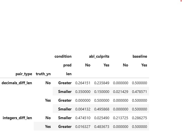
• Large gains for integers_equal_len and decimals_diff_len after ablation.
• surprisingly decimals_equal_len which can be compared as integers_equal_len for methodology of comparing as decimal has no effect when comparing.
• Even after ablation in decimals_diff_len, when truth is No and decimal part of the first number is greater in length, vs when decimal part of the first number is smaller in length it’s easier for model to predict when length is smaller vs length is greater which gives an indication that the model does take length of the values into account also.

Verification Findings
Results are not very different from the previous approach with similar trends.

6. Limitations & Possible Next steps:

• (a) Prompt diversity : Have analysed a single prompt. Can try for different types of prompts.
• (b) String Analysis : More exploration needed why strings were biased towards No.
• (c) Tokenization was not deeply analysed. Only observation was that every number and comparator operator was getting tokenized individually.
• (d) Didn’t try PCA post ablation to see how the geometry changes.
• (e) Work currently analyse only one model Gemma-2-2b-it. And also only instruction tuned model. A good study could have been how the last layer of non instruction tuned behaved vs the instruction tuned.
• (f) Doesn’t analyse negative numbers in comparison.

Appendix

A. Harmful neurons

Top 50 global harmful neurons

Global Top 50 harmful neurons: [ 406, 7592, 2045, 7026, 7986, 8945, 8673, 3809, 6040, 341, 6406, 3954, 3667, 4487, 1914, 4673, 530, 7188, 7870, 2177, 7472, 8579, 2482, 496, 2405, 5205, 6743, 6076, 2251, 8510, 3280, 721, 4015, 7248, 9126, 6726, 6968, 5980, 3294, 526, 2363, 8659, 1232, 6534, 3628, 7565, 4482, 6024, 8467, 5637]

Top 30 harmful neurons by dataset

Neurons more harmful in decimals_diff_len: [406, 7592, 7026, 2045, 7986, 8945, 8222, 6040, 6743, 6406, 7033, 4361, 341, 3954, 4673, 5637, 8673, 3062, 4482, 2686, 7188, 1494, 2177, 8389, 822, 7184, 3200, 239, 1986, 4331] Neurons more harmful in integer_equal_len: [406, 7592, 2045, 7026, 7986, 8673, 8945, 3809, 4487, 6040, 3667, 3954, 341, 6406, 9022, 7248, 4015, 2076, 7870, 1232, 496, 9126, 481, 5205, 2405, 1914, 6968, 3294, 721, 530] Neurons more harmful in decimal_equal_len: [406, 7592, 7026, 2045, 7986, 3809, 8673, 4487, 341, 3667, 7188, 9022, 8945, 6040, 3954, 4015, 6968, 6406, 4576, 496, 721, 2405, 7248, 9126, 7870, 7472, 3294, 1914, 5205, 8254] Neurons more harmful in integers_diff_len: [406, 7592, 2045, 7026, 7986, 8945, 8673, 530, 3809, 4673, 8579, 1914, 2251, 6406, 5437, 3667, 4504, 9037, 5980, 6076, 8659, 2375, 8510, 4361, 341, 5246, 2177, 6040, 5892, 4283]

Interestingly, if we take a intersection of top50 global neurons vs top30 each dataset neurons.

Least intersection is with decimals_diff_len = 17 Then Integer_diff_len = 22 then tied integer_equal_len and decimal_equal_len = 27

B. What is the Yes–No mean difference?

Let each example i have:

• activation vector: h_i (dimension d)
• label: y_i ∈ {Yes, No}

Class index sets

• S_Yes = { i : y_i = Yes }
• S_No = { i : y_i = No }

Class means

• mu_Yes = average of { h_i

  i ∈ S_Yes }

• mu_No = average of { h_i

  i ∈ S_No }

Yes–No mean difference vector

• Delta = mu_Yes − mu_No (a vector in ℝ^d)

Unit direction (simple linear probe)

• w = Delta /

  Delta

  _2 (normalize Delta to length 1)

Signed score of any activation h along this axis

• score(h) = dot(h, w) (positive ⇒ evidence for “Yes”, negative ⇒ “No”)

Separation magnitude along the axis

• separation =

  E[score(h)

  y=Yes] − E[score(h)

  y=No]

C. Harmful Neuron Finding

How do I rank the neurons from most harmful to least harmful?

• We focus on the last transformer block post which it goes to ln_head.
• Residual stream output(after attn + mlp skip connections): r = resid_post[L-1] (shape: d_model).
• MLP hidden activations: h = mlp_post[L-1] (shape: d_mlp).
• MLP output weight: W_out (shape: d_mlp × d_model).
• Readout direction (Yes–No): Δw = W_U[Yes] - W_U[No].

Logit Gap (Margin)

The Yes–No margin is:

m(r) = <LN(r), Δw>, where LN is the final layer norm.

---

We know, Based on taylor expansion of first order m(r + Δr) ~ m(r) + (g^T)*(Δr)

We compute the gradient of the margin w.r.t. the residual: g = ∂m / ∂r

The MLP update is: r = r_post = r_mid + mlp_post(r_mlp)

Since, we only want to check how mlp_neurons are affecting:

Δr ~ Δr_mlp Hence, to compute

Δr_mlp = h @ W_out = Σ_j (h_j * W_out[j])

Contribution of neuron j to the margin: c_j = h_j * (W_out[j] · g)

Basically trying out to see, h_j how strongly neuron j is firing and gradient projected weight measures how much the margin cares about the direction that neuron writes. So we only focus on neurons which are affecting neurons most.

Next step would be to multiply it by (1 if Yes else -1) to align by truth.

References

• Nanda, N., & Bloom, J. (2022). TransformerLens. GitHub repository. https://github.com/TransformerLensOrg/TransformerLens
• Alain, G., & Bengio, Y. (2016). Understanding intermediate layers using linear classifier probes. arXiv:1610.01644. https://arxiv.org/abs/1610.01644

Disclaimer

I only did this research in ~15 hours so there are lot of things unexplored and the quality of work can be significantly improved. Took a lot more time in writing than I expected (probably around 7 hours to refine ) .